3. Examples
3.1. G2/M cell cycle transition
The SBML2Julia GitHub repository contains a version of the Vinod et Novak model of the G2/M cell cycle transition. The model contains 13 species, 13 simulated observables, 24 parameters and 4 experimental conditions.
3.1.1. Using the Python API
The SBML2Julia problem can be created using the Python API (and assuming that the current working directory is the SBML2Julia root directory) via:
>>> import sbml2julia

>>> problem = sbml2julia.SBML2JuliaProblem('examples/Vinod_FEBS2015/Vinod_FEBS2015.yaml')
and solved by:
>>> problem.optimize()
The results are then available under problem.results, which returns a dictionary containing 'par_best' (the best found parameter set), 'species', 'observables', 'fval' (the negative log-likelihood) and 'chi2' (chi2 values of residuals). For example, to access the best parameter set, type:
>>> problem.results['x_best']
                Name    par_0   par_best  par_best_to_par_0
0            kDpEnsa   0.0500   0.048840           0.976807
1              kPhGw   1.0000   0.955727           0.955727
2             kDpGw1   0.2500   0.236274           0.945095
3             kDpGw2  10.0000   9.727009           0.972701
4              kWee1   0.0100   0.009697           0.969738
5              kWee2   0.9900   1.308203           1.321418
6             kPhWee   1.0000   1.064760           1.064760
7             kDpWee  10.0000  10.181804           1.018180
8           kCdc25_1   0.1000   0.135812           1.358117
9           kCdc25_2   0.9000   1.099638           1.221820
10          kPhCdc25   1.0000   0.961436           0.961436
11          kDpCdc25  10.0000   8.990541           0.899054
12          kDipEB55   0.0068   0.003400           0.500002
13          kAspEB55  57.0000  46.386552           0.813799
14               fCb   2.0000   1.999269           0.999634
15             jiWee   0.1000   0.199999           1.999988
16           fB55_wt   1.0000   0.967920           0.967920
17         fB55_iWee   0.9000   0.886548           0.985053
18       fB55_Cb_low   1.1000   1.066191           0.969265
19     fB55_pGw_weak   1.0000   0.971742           0.971742
20        kPhEnsa_wt   0.1000   0.100393           1.003933
21      kPhEnsa_iWee   0.1000   0.097819           0.978187
22    kPhEnsa_Cb_low   0.1000   0.101325           1.013248
23  kPhEnsa_pGw_weak   0.0900   0.090801           1.008902
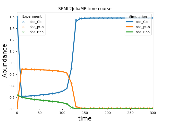
Selected observables of the optimized simulation of a given simulation condition can be plotted via:
>>> problem.plot_results(condition='wt', observables=['obs_Cb', 'obs_pCb', 'obs_B55'])
3.1.2. Using the command line interface
Similarly, the same example problem can be solved from the command line interface:
user@bash:/sbml2julia$ sbml2julia optimize 'examples/Vinod_FEBS2015/Vinod_FEBS2015.yaml' -d 'examples/Vinod_FEBS2015/results/'
The results can be found in the output directory given to the -d argument.
3.2. Gut microbial community
The SBML2Julia GitHub repository contains a generalised Lotka-Volterra model of 12 gut bacteria. The model conceived by Shin et al. contains 2 species, 2 observables, 156 parameters and 210 experimental conditions in its PEtab formulation.
3.2.1. Using the Python API
The SBML2Julia problem can be created using the Python API (and assuming that the current working directory is the sbml2julia root directory) via:
>>> import sbml2julia

>>> problem = sbml2julia.SBML2JuliaProblem('examples/Shin_PLOS2019/Shin_PLOS2019.yaml'})
and solved by:
>>> problem.optimize()
Again, the results are available under problem.results. Plots of the observables can be generated with the problem.plot_results() method and results can be written to TSV files with problem.write_results().
3.2.2. Using the command line interface
Similarly, the same example problem can be solved from the command line interface:
user@bash:/sbml2julia$ sbml2julia optimize 'examples/Shin_PLOS2019/Shin_PLOS2019.yaml' -d './examples/Shin_PLOS2019/results/'
The results can be found in the output directory given to the -d argument.